SENCE 2025 Examples¶

inselpy¶

• https://insel.eu/development/
• https://pypi.org/project/insel/

In [1]:

import insel
insel.block('sum', 2, 3)

import insel insel.block('sum', 2, 3)

Out[1]:

5.0

In [2]:

insel.block('do', parameters=[1, 10, 1])

insel.block('do', parameters=[1, 10, 1])

Out[2]:

[1.0, 2.0, 3.0, 4.0, 5.0, 6.0, 7.0, 8.0, 9.0, 10.0]

In [3]:

insel.block('gain', 2, 5, 7, parameters=[3], outputs=3)

insel.block('gain', 2, 5, 7, parameters=[3], outputs=3)

Out[3]:

[6.0, 15.0, 21.0]

In [4]:

insel.template('x_times_y.vseit', x=2, y=4)

insel.template('x_times_y.vseit', x=2, y=4)

Out[4]:

8.0

streamlit¶

https://streamlit.io/

# save to web_app.py
# run with: 
#   streamlit run my_web_app.py

import streamlit as st
import insel

st.title("INSEL online")
x = st.slider("X", 0, 100, 25)
y = st.slider("Y", 0, 100, 25)

result = insel.block('SUM', x, y)
st.write(f"{x} + {y} = {result}")

streamlit + INSEL templates¶

https://github.com/EricDuminil/streamlit_insel

import insel
import streamlit as st

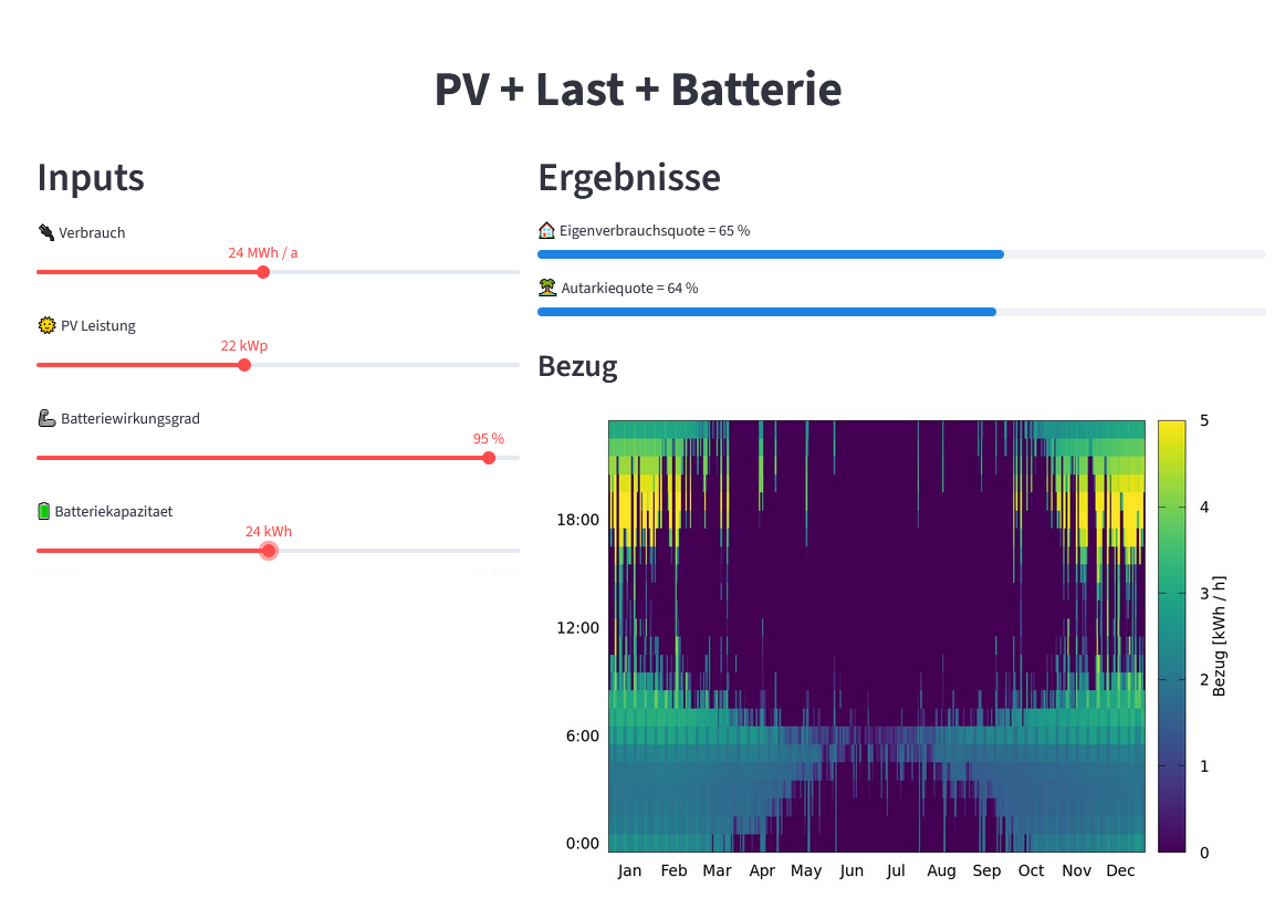
st.set_page_config(layout="wide", page_title="PV + Last + Batterie")
st.markdown(
    "<h1 style='text-align: center'>PV + Last + Batterie</h1>", unsafe_allow_html=True
)

left, right = st.columns([2, 3])

with left:
    st.header("Inputs")
    verbrauch = st.slider("🔌 Verbrauch", 1, 50, 10, format="%g MWh / a")
    pvleistung = st.slider("🌞 PV Leistung", 1, 50, 10, format="%g kWp")
    wirkungsgrad = st.slider("🦾 Batteriewirkungsgrad", 1, 100, 95, format="%g %%")
    kapazitaetbatterie = st.slider("🔋 Batteriekapazitaet", 0, 50, 5, format="%g kWh")

with right:
    st.header("Ergebnisse")
    eigenverbrauchsquote, autarkiequote, cycles = insel.template(
        "Last_PV_Batterie.vseit",
        MWh_Verbrauch=verbrauch,
        kWp_PV=pvleistung,
        Kapazitaet_Batterie=kapazitaetbatterie,
        Wirkungsgrad_Batterie=wirkungsgrad / 100,
    )

    st.progress(
        eigenverbrauchsquote,
        text=f"🏠 Eigenverbrauchsquote = {eigenverbrauchsquote*100:.0f} %",
    )

    st.progress(
        autarkiequote,
        text=f"🏝️ Autarkiequote = {autarkiequote*100:.0f} %",
    )

    st.badge(f"{cycles:.0f} Zyklen / a")
    st.subheader("Bezug")
    # NOTE: Could add a random id, for multi-users
    st.image("/tmp/Last_PV_Batterie.png")

random facts¶

In [5]:

import requests

# Example: API for a random fact
url = "https://uselessfacts.jsph.pl/random.json?language=en"
response = requests.get(url)

if response.status_code == 200:
    data = response.json()
    print("💡 Did you know?")
    print(data['text'])
else:
    print("Could not fetch the fact.")

import requests # Example: API for a random fact url = "https://uselessfacts.jsph.pl/random.json?language=en" response = requests.get(url) if response.status_code == 200: data = response.json() print("💡 Did you know?") print(data['text']) else: print("Could not fetch the fact.")

💡 Did you know?
Humans use a total of 72 different muscles in speech.

rich¶

In [6]:

from rich.progress import track
import time

for i in track(range(20), description="Hacking NASA..."):
    time.sleep(0.1)  # Simulate work

from rich.progress import track import time for i in track(range(20), description="Hacking NASA..."): time.sleep(0.1) # Simulate work

Output()

prettymapp¶

https://prettymapp.streamlit.app/

In [9]:

from prettymapp.geo import get_aoi
from prettymapp.osm import get_osm_geometries
from prettymapp.plotting import Plot
from prettymapp.settings import STYLES

aoi = get_aoi(
    # Location can either be defined by coordinates:
    coordinates=(45.43900, 12.32625),
    # or an address:
    # address="Praça Ferreira do Amaral, Macau",
    radius=1500,
    rectangular=False,
)

df = get_osm_geometries(aoi=aoi)

fig = Plot(
    df=df,
    aoi_bounds=aoi.bounds,
    draw_settings=STYLES["Citrus"],
    credits=False,
).plot_all()

fig.set_dpi(120)

# If you want to save it to a PNG file, with 3600x3600px
# fig.savefig("images/venice.png", dpi=300)

from prettymapp.geo import get_aoi from prettymapp.osm import get_osm_geometries from prettymapp.plotting import Plot from prettymapp.settings import STYLES aoi = get_aoi( # Location can either be defined by coordinates: coordinates=(45.43900, 12.32625), # or an address: # address="Praça Ferreira do Amaral, Macau", radius=1500, rectangular=False, ) df = get_osm_geometries(aoi=aoi) fig = Plot( df=df, aoi_bounds=aoi.bounds, draw_settings=STYLES["Citrus"], credits=False, ).plot_all() fig.set_dpi(120) # If you want to save it to a PNG file, with 3600x3600px # fig.savefig("images/venice.png", dpi=300)

Satellite images¶

https://github.com/EricDuminil/satellite-imagery-downloader

In [10]:

from IPython.display import Image
Image(filename='images/houat.png')

from IPython.display import Image Image(filename='images/houat.png')

Out[10]:

pandas¶

In [7]:

import pandas as pd

pd.read_csv('https://web.stanford.edu/class/archive/cs/cs109/cs109.1166/stuff/titanic.csv')

import pandas as pd pd.read_csv('https://web.stanford.edu/class/archive/cs/cs109/cs109.1166/stuff/titanic.csv')

Out[7]:

	Survived	Pclass	Name	Sex	Age	Siblings/Spouses Aboard	Parents/Children Aboard	Fare
0	0	3	Mr. Owen Harris Braund	male	22.0	1	0	7.2500
1	1	1	Mrs. John Bradley (Florence Briggs Thayer) Cum...	female	38.0	1	0	71.2833
2	1	3	Miss. Laina Heikkinen	female	26.0	0	0	7.9250
3	1	1	Mrs. Jacques Heath (Lily May Peel) Futrelle	female	35.0	1	0	53.1000
4	0	3	Mr. William Henry Allen	male	35.0	0	0	8.0500
...	...	...	...	...	...	...	...	...
882	0	2	Rev. Juozas Montvila	male	27.0	0	0	13.0000
883	1	1	Miss. Margaret Edith Graham	female	19.0	0	0	30.0000
884	0	3	Miss. Catherine Helen Johnston	female	7.0	1	2	23.4500
885	1	1	Mr. Karl Howell Behr	male	26.0	0	0	30.0000
886	0	3	Mr. Patrick Dooley	male	32.0	0	0	7.7500

887 rows × 8 columns

In [8]:

pd.read_csv('http://ultra.ericduminil.com/data/all_ultras.csv', sep=';')

pd.read_csv('http://ultra.ericduminil.com/data/all_ultras.csv', sep=';')

Out[8]:

	id	name	miles	division	laps	discipline	country	age	elapsed_time	kilometers	venue	year
0	miami_2025_151	Joe Mazzone	320.29200	Open	217	Push	US	30-39	23.92384	515.460	Miami Ultra	2025
1	miami_2021_49	Joe Mazzone	313.90000	Open	215	Push	US	30-39	23.64750	505.173	Miami Ultra	2021
2	dutch_2017_13	Rick Pronk	313.17108	Open	160	Push	NL	1-49	23.95963	504.000	Dutch Ultra	2017
3	dutch_2018_18	Rick Pronk	311.21376	Open	159	Push	NL	1-49	23.91601	500.850	Dutch Ultra	2018
4	miami_2016_201	Andrew Andras	309.52000	Open	212	Push	US	30-39	23.96444	498.124	Miami Ultra	2016
...	...	...	...	...	...	...	...	...	...	...	...	...
1569	miami_2015_256	Jennifer Gonzalez	7.30000	Women	5	Push	US	19-29	8.89917	11.748	Miami Ultra	2015
1570	miami_2019_26	Zack Knezevic	7.30000	Open	5	Push	US	30-39	17.43500	11.748	Miami Ultra	2019
1571	miami_2025_138	Scott Ziegler	5.90400	Open	4	Push	US	40-49	23.14916	9.502	Miami Ultra	2025
1572	miami_2022_132	Zack K	2.92000	Open	2	Push	World	40-49	13.85972	4.699	Miami Ultra	2022
1573	miami_2023_64	Leonard L Leffler	1.46000	Open	1	Paddle	US	50-59	23.00992	2.350	Miami Ultra	2023

1574 rows × 12 columns

Large data¶

Library: https://docs.xarray.dev/en/stable/

Data: https://berkeleyearth.org/data/ https://berkeley-earth-temperature.s3.us-west-1.amazonaws.com/Global/Gridded/Land_and_Ocean_LatLong1.nc

In [11]:

import xarray as xr

# from https://berkeleyearth.org/data/
ds = xr.open_dataset("~/Downloads/Land_and_Ocean_LatLong1.nc")

import xarray as xr # from https://berkeleyearth.org/data/ ds = xr.open_dataset("~/Downloads/Land_and_Ocean_LatLong1.nc")

In [12]:

ds

ds

Out[12]:

<xarray.Dataset>
Dimensions:      (longitude: 360, latitude: 180, time: 2100, month_number: 12)
Coordinates:
  * longitude    (longitude) float32 -179.5 -178.5 -177.5 ... 177.5 178.5 179.5
  * latitude     (latitude) float32 -89.5 -88.5 -87.5 -86.5 ... 87.5 88.5 89.5
  * time         (time) float64 1.85e+03 1.85e+03 ... 2.025e+03 2.025e+03
Dimensions without coordinates: month_number
Data variables:
    land_mask    (latitude, longitude) float64 ...
    temperature  (time, latitude, longitude) float32 ...
    climatology  (month_number, latitude, longitude) float32 ...
Attributes:
    Conventions:           Berkeley Earth Internal Convention (based on CF-1.5)
    title:                 Native Format Berkeley Earth Surface Temperature A...
    history:               09-Jan-2025 20:35:17
    institution:           Berkeley Earth Surface Temperature Project
    land_source_history:   04-Jan-2025 19:11:11
    ocean_source_history:  06-Jan-2025 11:47:59
    comment:               This file contains Berkeley Earth surface temperat...

xarray.Dataset

• Dimensions:
  • longitude: 360
  • latitude: 180
  • time: 2100
  • month_number: 12
• Coordinates: (3)
  • longitude
    (longitude)
    float32
    -179.5 -178.5 ... 178.5 179.5

    units :

    degrees_east

    standard_name :

    longitude

    long_name :

    Longitude

    array([-179.5, -178.5, -177.5, ...,  177.5,  178.5,  179.5], dtype=float32)

  • latitude
    (latitude)
    float32
    -89.5 -88.5 -87.5 ... 88.5 89.5

    units :

    degrees_north

    standard_name :

    latitude

    long_name :

    Latitude

    array([-89.5, -88.5, -87.5, -86.5, -85.5, -84.5, -83.5, -82.5, -81.5, -80.5,
           -79.5, -78.5, -77.5, -76.5, -75.5, -74.5, -73.5, -72.5, -71.5, -70.5,
           -69.5, -68.5, -67.5, -66.5, -65.5, -64.5, -63.5, -62.5, -61.5, -60.5,
           -59.5, -58.5, -57.5, -56.5, -55.5, -54.5, -53.5, -52.5, -51.5, -50.5,
           -49.5, -48.5, -47.5, -46.5, -45.5, -44.5, -43.5, -42.5, -41.5, -40.5,
           -39.5, -38.5, -37.5, -36.5, -35.5, -34.5, -33.5, -32.5, -31.5, -30.5,
           -29.5, -28.5, -27.5, -26.5, -25.5, -24.5, -23.5, -22.5, -21.5, -20.5,
           -19.5, -18.5, -17.5, -16.5, -15.5, -14.5, -13.5, -12.5, -11.5, -10.5,
            -9.5,  -8.5,  -7.5,  -6.5,  -5.5,  -4.5,  -3.5,  -2.5,  -1.5,  -0.5,
             0.5,   1.5,   2.5,   3.5,   4.5,   5.5,   6.5,   7.5,   8.5,   9.5,
            10.5,  11.5,  12.5,  13.5,  14.5,  15.5,  16.5,  17.5,  18.5,  19.5,
            20.5,  21.5,  22.5,  23.5,  24.5,  25.5,  26.5,  27.5,  28.5,  29.5,
            30.5,  31.5,  32.5,  33.5,  34.5,  35.5,  36.5,  37.5,  38.5,  39.5,
            40.5,  41.5,  42.5,  43.5,  44.5,  45.5,  46.5,  47.5,  48.5,  49.5,
            50.5,  51.5,  52.5,  53.5,  54.5,  55.5,  56.5,  57.5,  58.5,  59.5,
            60.5,  61.5,  62.5,  63.5,  64.5,  65.5,  66.5,  67.5,  68.5,  69.5,
            70.5,  71.5,  72.5,  73.5,  74.5,  75.5,  76.5,  77.5,  78.5,  79.5,
            80.5,  81.5,  82.5,  83.5,  84.5,  85.5,  86.5,  87.5,  88.5,  89.5],
          dtype=float32)

  • time
    (time)
    float64
    1.85e+03 1.85e+03 ... 2.025e+03

    units :

    year A.D.

    standard_name :

    time

    long_name :

    Time

    array([1850.041667, 1850.125   , 1850.208333, ..., 2024.791667, 2024.875   ,
           2024.958333])

• Data variables: (3)
  • land_mask
    (latitude, longitude)
    float64
    ...

    units :

    none

    standard_name :

    land_mask

    long_name :

    Land Mask

    valid_min :

    0.0

    valid_max :

    1.0

    [64800 values with dtype=float64]

  • temperature
    (time, latitude, longitude)
    float32
    ...

    units :

    degree C

    standard_name :

    surface_temperature_anomaly

    long_name :

    Air Surface Temperature Anomaly

    valid_min :

    -19.38505283824927

    valid_max :

    22.232753304325723

    [136080000 values with dtype=float32]

  • climatology
    (month_number, latitude, longitude)
    float32
    ...

    units :

    degree C

    standard_name :

    surface_temperature_climatology

    long_name :

    Air Surface Temperature Climatology (Jan 1951 - Dec 1980)

    valid_min :

    -65.3279208344876

    valid_max :

    36.720723102195144

    [777600 values with dtype=float32]

• Indexes: (3)
  • longitude
    PandasIndex

    PandasIndex(Index([-179.5, -178.5, -177.5, -176.5, -175.5, -174.5, -173.5, -172.5, -171.5,
           -170.5,
           ...
            170.5,  171.5,  172.5,  173.5,  174.5,  175.5,  176.5,  177.5,  178.5,
            179.5],
          dtype='float32', name='longitude', length=360))

  • latitude
    PandasIndex

    PandasIndex(Index([-89.5, -88.5, -87.5, -86.5, -85.5, -84.5, -83.5, -82.5, -81.5, -80.5,
           ...
            80.5,  81.5,  82.5,  83.5,  84.5,  85.5,  86.5,  87.5,  88.5,  89.5],
          dtype='float32', name='latitude', length=180))

  • time
    PandasIndex

    PandasIndex(Index([1850.0416666666667,           1850.125, 1850.2083333333333,
           1850.2916666666667,           1850.375, 1850.4583333333333,
           1850.5416666666667,           1850.625, 1850.7083333333333,
           1850.7916666666667,
           ...
           2024.2083333333333, 2024.2916666666665,           2024.375,
           2024.4583333333333, 2024.5416666666665,           2024.625,
           2024.7083333333333, 2024.7916666666665,           2024.875,
           2024.9583333333333],
          dtype='float64', name='time', length=2100))

• Attributes: (7)

  Conventions :

  Berkeley Earth Internal Convention (based on CF-1.5)

  title :

  Native Format Berkeley Earth Surface Temperature Anomaly Field

  history :

  09-Jan-2025 20:35:17

  institution :

  Berkeley Earth Surface Temperature Project

  land_source_history :

  04-Jan-2025 19:11:11

  ocean_source_history :

  06-Jan-2025 11:47:59

  comment :

  This file contains Berkeley Earth surface temperature anomaly field in our native equal-area format.

In [13]:

ds.sel(longitude=9, latitude=48.7, method='nearest')['temperature'].plot();

ds.sel(longitude=9, latitude=48.7, method='nearest')['temperature'].plot();

In [14]:

ds.sel(time=2003 + 7.5 / 12, method='nearest').sel(latitude=slice(35, 65), longitude=slice(-10,30))['temperature'].plot();

ds.sel(time=2003 + 7.5 / 12, method='nearest').sel(latitude=slice(35, 65), longitude=slice(-10,30))['temperature'].plot();

In [15]:

ds.climatology.sel(month_number=0).plot();

ds.climatology.sel(month_number=0).plot();

In [16]:

stuttgart = ds.sel(longitude=9, latitude=48.7, method='nearest')
stuttgart

stuttgart = ds.sel(longitude=9, latitude=48.7, method='nearest') stuttgart

Out[16]:

<xarray.Dataset>
Dimensions:      (time: 2100, month_number: 12)
Coordinates:
    longitude    float32 9.5
    latitude     float32 48.5
  * time         (time) float64 1.85e+03 1.85e+03 ... 2.025e+03 2.025e+03
Dimensions without coordinates: month_number
Data variables:
    land_mask    float64 ...
    temperature  (time) float32 ...
    climatology  (month_number) float32 ...
Attributes:
    Conventions:           Berkeley Earth Internal Convention (based on CF-1.5)
    title:                 Native Format Berkeley Earth Surface Temperature A...
    history:               09-Jan-2025 20:35:17
    institution:           Berkeley Earth Surface Temperature Project
    land_source_history:   04-Jan-2025 19:11:11
    ocean_source_history:  06-Jan-2025 11:47:59
    comment:               This file contains Berkeley Earth surface temperat...

xarray.Dataset

• Dimensions:
  • time: 2100
  • month_number: 12
• Coordinates: (3)
  • longitude
    ()
    float32
    9.5

    units :

    degrees_east

    standard_name :

    longitude

    long_name :

    Longitude

    array(9.5, dtype=float32)

  • latitude
    ()
    float32
    48.5

    units :

    degrees_north

    standard_name :

    latitude

    long_name :

    Latitude

    array(48.5, dtype=float32)

  • time
    (time)
    float64
    1.85e+03 1.85e+03 ... 2.025e+03

    units :

    year A.D.

    standard_name :

    time

    long_name :

    Time

    array([1850.041667, 1850.125   , 1850.208333, ..., 2024.791667, 2024.875   ,
           2024.958333])

• Data variables: (3)
  • land_mask
    ()
    float64
    ...

    units :

    none

    standard_name :

    land_mask

    long_name :

    Land Mask

    valid_min :

    0.0

    valid_max :

    1.0

    [1 values with dtype=float64]

  • temperature
    (time)
    float32
    ...

    units :

    degree C

    standard_name :

    surface_temperature_anomaly

    long_name :

    Air Surface Temperature Anomaly

    valid_min :

    -19.38505283824927

    valid_max :

    22.232753304325723

    [2100 values with dtype=float32]

  • climatology
    (month_number)
    float32
    ...

    units :

    degree C

    standard_name :

    surface_temperature_climatology

    long_name :

    Air Surface Temperature Climatology (Jan 1951 - Dec 1980)

    valid_min :

    -65.3279208344876

    valid_max :

    36.720723102195144

    [12 values with dtype=float32]

• Indexes: (1)
  • time
    PandasIndex

    PandasIndex(Index([1850.0416666666667,           1850.125, 1850.2083333333333,
           1850.2916666666667,           1850.375, 1850.4583333333333,
           1850.5416666666667,           1850.625, 1850.7083333333333,
           1850.7916666666667,
           ...
           2024.2083333333333, 2024.2916666666665,           2024.375,
           2024.4583333333333, 2024.5416666666665,           2024.625,
           2024.7083333333333, 2024.7916666666665,           2024.875,
           2024.9583333333333],
          dtype='float64', name='time', length=2100))

• Attributes: (7)

  Conventions :

  Berkeley Earth Internal Convention (based on CF-1.5)

  title :

  Native Format Berkeley Earth Surface Temperature Anomaly Field

  history :

  09-Jan-2025 20:35:17

  institution :

  Berkeley Earth Surface Temperature Project

  land_source_history :

  04-Jan-2025 19:11:11

  ocean_source_history :

  06-Jan-2025 11:47:59

  comment :

  This file contains Berkeley Earth surface temperature anomaly field in our native equal-area format.

In [17]:

import numpy as np

import numpy as np

In [18]:

months = (np.floor((stuttgart.time - np.floor(stuttgart.time))*12)).astype(int)

months = (np.floor((stuttgart.time - np.floor(stuttgart.time))*12)).astype(int)

In [19]:

df = pd.DataFrame({
              'year': np.floor(stuttgart.time).astype(int),
              'month': months + 1,
              'temperature': stuttgart.climatology[months] + stuttgart.temperature,
             },            
            )
df

df = pd.DataFrame({ 'year': np.floor(stuttgart.time).astype(int), 'month': months + 1, 'temperature': stuttgart.climatology[months] + stuttgart.temperature, }, ) df

Out[19]:

	year	month	temperature
0	1850	1	-2.558053
1	1850	2	5.262820
2	1850	3	2.164932
3	1850	4	8.349158
4	1850	5	10.533581
...	...	...	...
2095	2024	8	20.524185
2096	2024	9	15.114173
2097	2024	10	12.679502
2098	2024	11	7.373162
2099	2024	12	4.583126

2100 rows × 3 columns

In [20]:

df.to_csv('output/stuttgart_monthly_temperatures.csv', index=False, sep='\t')

df.to_csv('output/stuttgart_monthly_temperatures.csv', index=False, sep='\t')

Edward R. Tufte, The Visual Display of Quantitative Information¶

Book: https://www.edwardtufte.com/book/the-visual-display-of-quantitative-information/

Examples: https://www.ajnisbet.com/blog/tufte-in-matplotlib

In [21]:

# From https://www.ajnisbet.com/blog/tufte-in-matplotlib

import matplotlib.pyplot as plt
import matplotlib.ticker as ticker

# Global options.
plt.rcParams['font.family'] = 'serif'

# Data from p74 of Visual Display of Quantitative Information.
x = list(range(1951, 1960))
y = [264, 231, 274, 241, 322, 286, 283, 247, 243]

# Plot line, line masks, then dots.
fig, ax = plt.subplots()
ax.plot(x, y, linestyle='-', color='black', linewidth=1, zorder=1)
ax.scatter(x, y, color='white', s=100, zorder=2)
ax.scatter(x, y, color='black', s=20, zorder=3)

# Remove axis lines.
ax.spines['top'].set_visible(False)
ax.spines['right'].set_visible(False)

# Set spine extent.
ax.spines['bottom'].set_bounds(min(x), max(x))
ax.spines['left'].set_bounds(225, 325)

# Reduce tick spacing.
x_ticks = list(range(min(x), max(x)+1, 2))
ax.xaxis.set_ticks(x_ticks)
ax.yaxis.set_major_locator(ticker.MultipleLocator(base=25))
ax.tick_params(direction='in')

# Adjust lower limits to let data breathe.
ax.set_xlim([1950, ax.get_xlim()[1]])
ax.set_ylim([210, ax.get_ylim()[1]])

# Axis labels as a title annotation.
ax.text(1958, 320, 'Connecticut Traffic Deaths,\n1951 - 1959')
plt.show();

# From https://www.ajnisbet.com/blog/tufte-in-matplotlib import matplotlib.pyplot as plt import matplotlib.ticker as ticker # Global options. plt.rcParams['font.family'] = 'serif' # Data from p74 of Visual Display of Quantitative Information. x = list(range(1951, 1960)) y = [264, 231, 274, 241, 322, 286, 283, 247, 243] # Plot line, line masks, then dots. fig, ax = plt.subplots() ax.plot(x, y, linestyle='-', color='black', linewidth=1, zorder=1) ax.scatter(x, y, color='white', s=100, zorder=2) ax.scatter(x, y, color='black', s=20, zorder=3) # Remove axis lines. ax.spines['top'].set_visible(False) ax.spines['right'].set_visible(False) # Set spine extent. ax.spines['bottom'].set_bounds(min(x), max(x)) ax.spines['left'].set_bounds(225, 325) # Reduce tick spacing. x_ticks = list(range(min(x), max(x)+1, 2)) ax.xaxis.set_ticks(x_ticks) ax.yaxis.set_major_locator(ticker.MultipleLocator(base=25)) ax.tick_params(direction='in') # Adjust lower limits to let data breathe. ax.set_xlim([1950, ax.get_xlim()[1]]) ax.set_ylim([210, ax.get_ylim()[1]]) # Axis labels as a title annotation. ax.text(1958, 320, 'Connecticut Traffic Deaths,\n1951 - 1959') plt.show();

https://quarto.org/docs/gallery/ ?

CityGML ?¶

https://transfer.hft-stuttgart.de/gitlab/eric.duminil/get-bw-opendata

marimo?¶

• https://marimo.io/
• https://koaning.github.io/drawdata/
• https://martidossi.github.io/a-data-story/apps/1_when_european_fly_nest.html ?

pyvista?¶

https://docs.pyvista.org/